Hello! This summer I worked as one of the education interns, working with Mine Çetinkaya-Rundel and Garrett Grolemund on the RStudio Cheatsheets. I’m excited to share my work from this summer. Many RStudio cheatsheets have been updated or reworked based on recent package updates, and we’ve updated the cheatsheet contribution process as well. You’ll also see some small changes to the cheatsheet website reflecting these changes.

RStudio Cheatsheet Updates

Cheatsheets for dplyr, ggplot2, lubridate, forcats, reticulate, the RStudio IDE, Shiny, and stringr have been updated to reflect the most recent package updates. This includes dplyr’s row-wise grouping, the RStudio Visual Editor, and more.

R Markdown and Apply functions with purrr received more substantial redesigns. R Markdown was updated to match the new hex sticker colors and include new features related to the RStudio IDE Visual Editor. With the addition of row-wise grouping to dplyr, the list-column workflow on the previous purrr cheatsheet also needed to be updated and was moved to a new cheatsheet featuring tidyr and nested data. The new purrr cheatsheet focuses more on the many different map() functions available in the package on the first page, and all of the more general list functions on the second page.

Speaking of new cheatsheets, tidyr now has it’s own cheatsheet! Data tidying with tidyr features an overview of tibbles and how to reshape and work with tidy data on the first page, and a redesign of the nested data and list-column workflow from the previous purrr cheatsheet on the second page. The new page provides an overview of creating, reshaping, and transforming nested data and list-columns with tidyr, tibble, and dplyr. Previously tidyr was featured on the second page of the Data import with tidyr cheatsheet, and with the space provided by this change Data import with readr, readxl, and googlesheets4 now includes a second page covering spreadsheets, with readxl and googlesheets4.

See all of the current RStudio cheatsheets, as well as user contributed cheatsheets and translations on the RStudio website.

New Contribution Process

Another big project completed during my internship was reworking the process for handling user contributed cheatsheets. The Cheatsheet GitHub Repository now includes a Contributing Guidelines page outlining how to submit a new cheatsheet, or a new or updated translation. Both can now be submitted directly to GitHub via pull request, and you’ll see a template outlining everything to include.

Questions on the cheatsheets can now be submitted as issues on the Cheatsheet GitHub Repository. We have included issue templates to help guide this process, which can be particularly helpful if you’re new to GitHub. Just go to the Issues tab and choose the option that’s most relevant to your question!

Call for Translations

If you’re interested in translating a cheatsheet, please feel free to submit any updates using the new process! With the changes to so many cheatsheets, many translations would benefit from updates as well.

We really appreciate the work and care that goes into these translations. The first eight cheatsheets mentioned could be great starting points if you’re new to the process, since the changes were much smaller, and for many languages will require updating existing translations, instead of starting from scratch. If you’re interested in translating a cheatsheet, but have limited time or aren’t sure where to start, we’ve listed cheatsheets in each language that we think would be good first contributions as issues in the GitHub repo.

Happy summer from the R Markdown family! We are proud to share that bookdown (https://pkgs.rstudio.com/bookdown/) version 0.23 is on CRAN. bookdown is a package that helps you write books and long-form articles/reports, knitting together content from single or multiple R Markdown files as input.

Latest release

You can install bookdown from CRAN with:

install.packages("bookdown")
# or if the v0.23 binary package for your platform is not ready yet, try
# install.packages("bookdown", type = "source")

In this post, we’ll share some highlights from the latest release, but you might want to look at the release notes for the full details.

New HTML book format based on Bootstrap 4

This release includes a new HTML book output format called bs4_book(), contributed by Hadley Wickham and Maëlle Salmon. Based on Bootstrap 4, bs4_book() includes carefully crafted features to provide a clean reading experience whether you are on a phone, tablet, or desktop. On a full-size screen, the layout includes three columns of content so readers can quickly see all chapters on the left, the current chapter in the middle, and sections within the the current chapter on the right. As an example, you can read a book using this format here: https://mastering-shiny.org

Figure 1: Screenshot of a bs4_book home page.

Learn more about the unique features of this output format in the book “bookdown: Authoring Books and Technical Documents with R Markdown”: https://bookdown.org/yihui/bookdown/html.html#bs4-book

Our package reference site also has a documentation page for bs4_book(): https://pkgs.rstudio.com/bookdown/reference/bs4_book.html

New project template

To make it easier for users to start new bookdown book projects, we added two functions to create new bookdown projects:

• create_gitbook(), and
• create_bs4_book().

If you use RStudio, you can also access these two templates interactively from the New Project Wizard using File > New Project > New Directory.

Figure 2: Screenshot of the RStudio Project Wizard for creating a new bookdown project.

To help you build a new bookdown project faster, we also added some helpful pointers inside the template book itself to get you writing your book more quickly. You can think of the boilerplate content as a cheat sheet for the most useful features of bookdown so that you can easily access them if you are offline, or if you simply don’t have the docs right in front of you as you work. For example, you’ll find:

1. How to use parts, chapters, sections, and subsections to organize your content.
2. How to use cross-references, including to captioned figures and tables.
3. How to add footnotes and citations.
4. How to use custom blocks for equations, theorems and proofs, and callouts.
5. How to prepare your book to be shared.

We also included a _common.R script in the template project. By using before_chapter_script in your bookdown.yml file, this script is run at the beginning of each chapter:

before_chapter_script: _common.R

Importantly, this works with new_session: true since bookdown v0.18 (see news).

We hope these templates make it easier to start a book with bookdown. As always, with any template, you can also just cut out the template contents and start customizing and writing straight away too - the overall file structure and YAML configurations will still provide a useful skeleton for your next book.

output:
  bookdown::gitbook:
    config:
      search:
        engine: fuse # lunr is the default
        options: null # can override, see: https://fusejs.io/api/options.html

Each person’s genome, which collectively encodes the biochemical machinery they are born with, is composed of over 3 billion letters of DNA. However, only a small subset of the genome (~4-5 million positions) varies between two people. Nonetheless, each person’s unique genome interacts with the environment they experience to determine the majority of their health outcomes. A key method of understanding the relationship between genetic variants and traits is a genome-wide association study (GWAS), in which each genetic variant present in a cohort is individually examined for correlation with the trait of interest. GWAS results can be used to identify and prioritize potential therapeutic targets by identifying genes that are strongly associated with a disease of interest, and can also be used to build a polygenic risk score (PRS) to predict disease predisposition based on the combined influence of variants present in an individual. However, while accurate measurement of traits in an individual (called phenotyping) is essential to GWAS, it often requires painstaking expert curation and/or subjective judgment calls.

In “Large-scale machine learning-based phenotyping significantly improves genomic discovery for optic nerve head morphology”, we demonstrate how using machine learning (ML) models to classify medical imaging data can be used to improve GWAS. We describe how models can be trained for phenotypes to generate trait predictions and how these predictions are used to identify novel genetic associations. We then show that the novel associations discovered improve PRS accuracy and, using glaucoma as an example, that the improvements for anatomical eye traits relate to human disease. We have released the model training code and detailed documentation for its use on our Genomics Research GitHub repository.

Identifying genetic variants associated with eye anatomical traits
Previous work has demonstrated that ML models can identify eye diseases, skin diseases, and abnormal mammogram results with accuracy approaching or exceeding state-of-the-art methods by domain experts. Because identifying disease is a subset of phenotyping, we reasoned that ML models could be broadly used to improve the speed and quality of phenotyping for GWAS.

To test this, we chose a model that uses a fundus image of the eye to accurately predict whether a patient should be referred for assessment for glaucoma. This model uses the fundus images to predict the diameters of the optic disc (the region where the optic nerve connects to the retina) and the optic cup (a whitish region in the center of the optic disc). The ratio of the diameters of these two anatomical features (called the vertical cup-to-disc ratio, or VCDR) correlates strongly with glaucoma risk.

A representative retinal fundus image showing the vertical cup-to-disc ratio, which is an important diagnostic measurement for glaucoma.

We applied this model to predict VCDR in all fundus images from individuals in the UK Biobank, which is the world’s largest dataset available to researchers worldwide for health-related research in the public interest, containing extensive phenotyping and genetic data for ~500,000 pseudonymized (the UK Biobank's standard for de-identification) individuals. We then performed GWAS in this dataset to identify genetic variants that are associated with the model-based predictions of VCDR.

Applying a VCDR prediction model trained on clinical data to generate predicted values for VCDR to enable discovery of genetic associations for the VCDR trait.

The ML-based GWAS identified 156 distinct genomic regions associated with VCDR. We compared these results to a VCDR GWAS conducted by another group on the same UK Biobank data, Craig et al. 2020, where experts had painstakingly labeled all images for VCDR. The ML-based GWAS replicates 62 of the 65 associations found in Craig et al., which indicates that the model accurately predicts VCDR in the UK Biobank images. Additionally, the ML-based GWAS discovered 93 novel associations.

Number of statistically significant GWAS associations discovered by exhaustive expert labeling approach (Craig et al., left), and by our ML-based approach (right), with shared associations in the middle.

The ML-based GWAS improves polygenic model predictions
To validate that the novel associations discovered in the ML-based GWAS are biologically relevant, we developed independent PRSes using the Craig et al. and ML-based GWAS results, and tested their ability to predict human-expert-labeled VCDR in a subset of UK Biobank as well as a fully independent cohort (EPIC-Norfolk). The PRS developed from the ML-based GWAS showed greater predictive ability than the PRS built from the expert labeling approach in both datasets, providing strong evidence that the novel associations discovered by the ML-based method influence VCDR biology, and suggesting that the improved phenotyping accuracy (i.e., more accurate VCDR measurement) of the model translates into a more powerful GWAS.

The correlation between a polygenic risk score (PRS) for VCDR generated from the ML-based approach and the exhaustive expert labeling approach (Craig et al.). In these plots, higher values on the y-axis indicate a greater correlation and therefore greater prediction from only the genetic data. [* — p ≤ 0.05; *** — p ≤ 0.001]

As a second validation, because we know that VCDR is strongly correlated with glaucoma, we also investigated whether the ML-based PRS was correlated with individuals who had either self-reported that they had glaucoma or had medical procedure codes suggestive of glaucoma or glaucoma treatment. We found that the PRS for VCDR determined using our model predictions were also predictive of the probability that an individual had indications of glaucoma. Individuals with a PRS 2.5 or more standard deviations higher than the mean were more than 3 times as likely to have glaucoma in this cohort. We also observed that the VCDR PRS from ML-based phenotypes was more predictive of glaucoma than the VCDR PRS produced from the extensive manual phenotyping.

The odds ratio of glaucoma (self-report or ICD code) stratified by the PRS for VCDR determined using the ML-based phenotypes (in standard deviations from the mean). In this plot, the y-axis shows the probability that the individual has glaucoma relative to the baseline rate (represented by the dashed line). The x-axis shows standard deviations from the mean for the PRS. Data are visualized as a standard box plot, which illustrates values for the mean (the orange line), first and third quartiles, and minimum and maximum.

Conclusion
We have shown that ML models can be used to quickly phenotype large cohorts for GWAS, and that these models can increase statistical power in such studies. Although these examples were shown for eye traits predicted from retinal imaging, we look forward to exploring how this concept could generally apply to other diseases and data types.

Acknowledgments
We would like to especially thank co-author Dr. Anthony Khawaja of Moorfields Eye Hospital for contributing his extensive medical expertise. We also recognize the efforts of Professor Jamie Craig and colleagues for their exhaustive labeling of UK Biobank images, which allowed us to make comparisons with our method. Several authors of that work, as well as Professor Stuart MacGregor and collaborators in Australia and at Max Kelsen have independently replicated these findings, and we value these scientific contributions as well. Last, this work summarizes the work of the following Google contributors, who we would like to thank: Babak Alipanahi, Farhad Hormozdiari, Babak Behsaz, Justin Cosentino, Zachary R. McCaw, Emanuel Schorsch, D. Sculley, Elizabeth H. Dorfman, Sonia Phene, Naama Hammel, Andrew Carroll, and Cory Y. McLean

Melodies stuck in your head, often referred to as “earworms,” are a well-known and sometimes irritating phenomenon — once that earworm is there, it can be tough to get rid of it. Research has found that engaging with the original song, whether that’s listening to or singing it, will drive the earworm away. But what if you can’t quite recall the name of the song, and can only hum the melody?

Existing methods to match a hummed melody to its original polyphonic studio recording face several challenges. With lyrics, background vocals and instruments, the audio of a musical or studio recording can be quite different from a hummed tune. By mistake or design, when someone hums their interpretation of a song, often the pitch, key, tempo or rhythm may vary slightly or even significantly. That’s why so many existing approaches to query by humming match the hummed tune against a database of pre-existing melody-only or hummed versions of a song, instead of identifying the song directly. However, this type of approach often relies on a limited database that requires manual updates.

Launched in October, Hum to Search is a new fully machine-learned system within Google Search that allows a person to find a song using only a hummed rendition of it. In contrast to existing methods, this approach produces an embedding of a melody from a spectrogram of a song without generating an intermediate representation. This enables the model to match a hummed melody directly to the original (polyphonic) recordings without the need for a hummed or MIDI version of each track or for other complex hand-engineered logic to extract the melody. This approach greatly simplifies the database for Hum to Search, allowing it to constantly be refreshed with embeddings of original recordings from across the world — even the latest releases.

Background
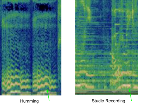
Many existing music recognition systems convert an audio sample into a spectrogram before processing it, in order to find a good match. However, one challenge in recognizing a hummed melody is that a hummed tune often contains relatively little information, as illustrated by this hummed example of Bella Ciao. The difference between the hummed version and the same segment from the corresponding studio recording can be visualized using spectrograms, seen below:

Visualization of a hummed clip and a matching studio recording.

Given the image on the left, a model needs to locate the audio corresponding to the right-hand image from a collection of over 50M similar-looking images (corresponding to segments of studio recordings of other songs). To achieve this, the model has to learn to focus on the dominant melody, and ignore background vocals, instruments, and voice timbre, as well as differences stemming from background noise or room reverberations. To find by eye the dominant melody that might be used to match these two spectrograms, a person might look for similarities in the lines near the bottom of the above images.

Prior efforts to enable discovery of music, in particular in the context of recognizing recorded music being played in an environment such as a cafe or a club, demonstrated how machine learning might be applied to this problem. Now Playing, released to Pixel phones in 2017, uses an on-device deep neural network to recognize songs without the need for a server connection, and Sound Search further developed this technology to provide a server-based recognition service for faster and more accurate searching of over 100 million songs. The next challenge then was to leverage what was learned from these releases to recognize hummed or sung music from a similarly large library of songs.

Machine Learning Setup
The first step in developing Hum to Search was to modify the music-recognition models used in Now Playing and Sound Search to work with hummed recordings. In principle, many such retrieval systems (e.g., image recognition) work in a similar way. A neural network is trained with pairs of input (here pairs of hummed or sung audio with recorded audio) to produce embeddings for each input, which will later be used for matching to a hummed melody.

Training setup for the neural network

To enable humming recognition, the network should produce embeddings for which pairs of audio containing the same melody are close to each other, even if they have different instrumental accompaniment and singing voices. Pairs of audio containing different melodies should be far apart. In training, the network is provided such pairs of audio until it learns to produce embeddings with this property.

The trained model can then generate an embedding for a tune that is similar to the embedding of the song’s reference recording. Finding the correct song is then only a matter of searching for similar embeddings from a database of reference recordings computed from audio of popular music.

Training Data
Because training of the model required song pairs (recorded and sung), the first challenge was to obtain enough training data. Our initial dataset consisted of mostly sung music segments (very few of these contained humming). To make the model more robust, we augmented the audio during training, for example by varying the pitch or tempo of the sung input randomly. The resulting model worked well enough for people singing, but not for people humming or whistling.

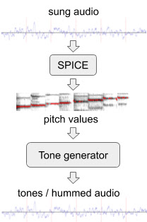
To improve the model’s performance on hummed melodies we generated additional training data of simulated “hummed” melodies from the existing audio dataset using SPICE, a pitch extraction model developed by our wider team as part of the FreddieMeter project. SPICE extracts the pitch values from given audio, which we then use to generate a melody consisting of discrete audio tones. The very first version of this system transformed this original clip into these tones.

Generating hummed audio from sung audio

We later refined this approach by replacing the simple tone generator with a neural network that generates audio resembling an actual hummed or whistled tune. For example, the network generates this humming example or whistling example from the above sung clip.

As a final step, we compared training data by mixing and matching the audio samples. For example, if we had a similar clip from two different singers, we’d align those two clips with our preliminary models, and are therefore able to show the model an additional pair of audio clips that represent the same melody.

Machine Learning Improvements
When training the Hum to Search model, we started with a triplet loss function. This loss has been shown to perform well across a variety of classification tasks like images and recorded music. Given a pair of audio corresponding to the same melody (corresponding to points R and P in embedding space shown below), triplet loss would ignore certain parts of the training data derived from a different melody. This helps the machine improve learning behavior, either when it finds a different melody that is too ‘easy’ in that it is already far away from R and P (see point E) or because it is too hard in that, given its current state of learning, the audio ends up being too close to R — even though according to our data it represents a different melody (see point H).

Example audio segments visualized as points in embedding space

We’ve found that we could improve the accuracy of our model by taking these additional training data (points H and E) into account, namely by formulating a general notion of model confidence across a batch of examples: How sure is the model that all the data it has seen can be classified correctly, or has it seen examples that do not fit its current understanding? Based on this notion of confidence, we added a loss that drives model confidence towards 100% across all areas of the embedding space, which led to improvements in our model’s precision and recall.

The above changes, but in particular our variations, augmentations and superpositions of the training data, enabled the neural network model deployed in Google Search to recognize sung or hummed melodies. The current system reaches a high level of accuracy on a song database that contains over half a million songs that we are continually updating. This song corpus still has room to grow to include more of the world’s many melodies.

Hum to Search in the Google App

To try the feature, you can open the latest version of the Google app, tap the mic icon and say “what's this song?” or click the “Search a song” button, after which you can hum, sing, or whistle away! We hope that Hum to Search can help with that earworm of yours, or maybe just help you in case you want to find and playback a song without having to type its name.

Acknowledgements
The work described here was authored by Alex Tudor, Duc Dung Nguyen, Matej Kastelic‎, Mihajlo Velimirović‎, Stefan Christoph, Mauricio Zuluaga, Christian Frank, Dominik Roblek, and Matt Sharifi. We would like to deeply thank Krishna Kumar, Satyajeet Salgar and Blaise Aguera y Arcas for their ongoing support, as well as all the Google teams we've collaborated with to build the full Hum to Search product.

We would also like to thank all our colleagues at Google who donated clips of themselves singing or humming and therefore laid a foundation for this work, as well as Nick Moukhine‎ for building the Google-internal singing donation app. Finally, special thanks to Meghan Danks and Krishna Kumar for their feedback on earlier versions of this post.

While tremendous efforts are invested in improving the quality of videos taken with smartphone cameras, the quality of audio in videos is often overlooked. For example, the speech of a subject in a video where there are multiple people speaking or where there is high background noise might be muddled, distorted, or difficult to understand. In an effort to address this, two years ago we introduced “Looking to Listen”, a machine learning (ML) technology that uses both visual and audio cues to isolate the speech of a video’s subject. By training the model on a large-scale collection of online videos, we are able to capture correlations between speech and visual signals such as mouth movements and facial expressions, which can then be used to separate the speech of one person in a video from another, or to separate speech from background sounds. We showed that this technology not only achieves state-of-the-art results in speech separation and enhancement (a noticeable 1.5dB improvement over audio-only models), but in particular can improve the results over audio-only processing when there are multiple people speaking, as the visual cues in the video help determine who is saying what.

We are now happy to make the Looking-to-Listen technology available to users through a new audiovisual Speech Enhancement feature in YouTube Stories (on iOS), allowing creators to take better selfie videos by automatically enhancing their voices and reducing background noise. Getting this technology into users’ hands was no easy feat. Over the past year, we worked closely with users to learn how they would like to use such a feature, in what scenarios, and what balance of speech and background sounds they would like to have in their videos. We heavily optimized the Looking-to-Listen model to make it run efficiently on mobile devices, overall reducing the running time from 10x real-time on a desktop when our paper came out, to 0.5x real-time performance on the phone. We also put the technology through extensive testing to verify that it performs consistently across different recording conditions and for people with different appearances and voices.

From Research to Product
Optimizing Looking-to-Listen to allow fast and robust operation on mobile devices required us to overcome a number of challenges. First, all processing needed to be done on-device within the client app in order to minimize processing time and to preserve the user’s privacy; no audio or video information would be sent to servers for processing. Further, the model needed to co-exist alongside other ML algorithms used in the YouTube app in addition to the resource-consuming video recording itself. Finally, the algorithm needed to run quickly and efficiently on-device while minimizing battery consumption.

The first step in the Looking-to-Listen pipeline is to isolate thumbnail images that contain the faces of the speakers from the video stream. By leveraging MediaPipe BlazeFace with GPU accelerated inference, this step is now able to be executed in just a few milliseconds. We then switched the model part that processes each thumbnail separately to a lighter weight MobileNet (v2) architecture, which outputs visual features learned for the purpose of speech enhancement, extracted from the face thumbnails in 10 ms per frame. Because the compute time to embed the visual features is short, it can be done while the video is still being recorded. This avoids the need to keep the frames in memory for further processing, thereby reducing the overall memory footprint. Then, after the video finishes recording, the audio and the computed visual features are streamed to the audio-visual speech separation model which produces the isolated and enhanced speech.

We reduced the total number of parameters in the audio-visual model by replacing “regular” 2D convolutions with separable ones (1D in the frequency dimension, followed by 1D in the time dimension) with fewer filters. We then optimized the model further using TensorFlow Lite — a set of tools that enable running TensorFlow models on mobile devices with low latency and a small binary size. Finally, we reimplemented the model within the Learn2Compress framework in order to take advantage of built-in quantized training and QRNN support.

Our Looking-to-Listen on-device pipeline for audiovisual speech enhancement

These optimizations and improvements reduced the running time from 10x real-time on a desktop using the original formulation of Looking-to-Listen, to 0.5x real-time performance using only an iPhone CPU; and brought the model size down from 120MB to 6MB now, which makes it easier to deploy. Since YouTube Stories videos are short — limited to 15 seconds — the result of the video processing is available within a couple of seconds after the recording is finished.

Finally, to avoid processing videos with clean speech (so as to avoid unnecessary computation), we first run our model only on the first two seconds of the video, then compare the speech-enhanced output to the original input audio. If there is sufficient difference (meaning the model cleaned up the speech), then we enhance the speech throughout the rest of the video.

Researching User Needs
Early versions of Looking-to-Listen were designed to entirely isolate speech from the background noise. In a user study conducted together with YouTube, we found that users prefer to leave in some of the background sounds to give context and to retain some the general ambiance of the scene. Based on this user study, we take a linear combination of the original audio and our produced clean speech channel: output_audio = 0.1 x original_audio + 0.9 x speech. The following video presents clean speech combined with different levels of the background sounds in the scene (10% background is the balance we use in practice).

Below are additional examples of the enhanced speech results from the new Speech Enhancement feature in YouTube Stories. We recommend watching the videos with good speakers or headphones.

Fairness Analysis
Another important requirement is that the model be fair and inclusive. It must be able to handle different types of voices, languages and accents, as well as different visual appearances. To this end, we conducted a series of tests exploring the performance of the model with respect to various visual and speech/auditory attributes: the speaker’s age, skin tone, spoken language, voice pitch, visibility of the speaker’s face (% of video in which the speaker is in frame), head pose throughout the video, facial hair, presence of glasses, and the level of background noise in the (input) video.

For each of the above visual/auditory attributes, we ran our model on segments from our evaluation set (separate from the training set) and measured the speech enhancement accuracy, broken down according to the different attribute values. Results for some of the attributes are summarized in the following plots. Each data point in the plots represents hundreds (in most cases thousands) of videos fitting the criteria.

Speech enhancement quality (signal-to-distortion ratio, SDR, in dB) for different spoken languages, sorted alphabetically. The average SDR was 7.89 dB with a standard deviation of 0.42 dB — deviation that for human listeners is considered hard to notice.

Left: Speech enhancement quality as a function of the speaker’s voice pitch. The fundamental voice frequency (pitch) of an adult male typically ranges from 85 to 180 Hz, and that of an adult female ranges from 165 to 255 Hz. Right: speech enhancement quality as a function of the speaker’s predicted age.

As our method utilizes facial cues and mouth movements to isolate the speech, we tested whether facial hair (e.g., a moustache, beard) may obstruct those visual cues and affect the method’s performance. Our evaluations show that the quality of speech enhancement is maintained well also in the presence of facial hair.

Using the Feature
YouTube creators who are eligible for YouTube Stories creation may record a video on iOS, and select “Enhance speech” from the volume controls editing tool. This will immediately apply speech enhancement to the audio track and will play back the enhanced speech in a loop. It is then possible to toggle the feature on and off multiple times to compare the enhanced speech with the original audio.

In parallel to this new feature in YouTube, we are also exploring additional venues for this technology. More to come later this year — stay tuned!

Acknowledgements
This feature is a collaboration across multiple teams at Google. Key contributors include: from Research-IL: Oran Lang; from VisCAM: Ariel Ephrat, Mike Krainin, JD Velasquez, Inbar Mosseri, Michael Rubinstein; from Learn2Compress: Arun Kandoor; from MediaPipe: Buck Bourdon, Matsvei Zhdanovich, Matthias Grundmann; from YouTube: Andy Poes, Vadim Lavrusik, Aaron La Lau, Willi Geiger, Simona De Rosa, and Tomer Margolin.

Microsoft has released a GitHub repository to share best practices for time series forecasting. From the repo:

Time series forecasting is one of the most important topics in data science. Almost every business needs to predict the future in order to make better decisions and allocate resources more effectively.

This repository provides examples and best practice guidelines for building forecasting solutions. The goal of this repository is to build a comprehensive set of tools and examples that leverage recent advances in forecasting algorithms to build solutions and operationalize them. Rather than creating implementations from scratch, we draw from existing state-of-the-art libraries and build additional utilities around processing and featurizing the data, optimizing and evaluating models, and scaling up to the cloud.

The repository includes detailed examples of various time series modeling techniques, as Jupyter Notebooks for Python, and R Markdown documents for R. It also includes Python notebooks to fit time series models in the Azure Machine Learning service, and then operationalize the forecasts as a web service.

The R examples demonstrate several techniques for forecasting time series, specifically data on refrigerated orange juice sales from 83 stores (sourced from the the bayesm package). The forecasting techniques vary (mean forecasting with interpolation, ARIMA, exponential smoothing, and additive models), but all make extensive use of the tidyverts suite of packages, which provides "tidy time series forecasting for R". The forecasting methods themselves are explained in detail in the book (readable online) Forecasting: Principles and Practice by Rob J Hyndman and George Athanasopoulos (Monash University).

You can try out the examples yourself by cloning the repository and knitting the RMarkdown files in R. If you have git installed, a quick and easy way to do this in with RStudio. Choose File > New Project > Version Control > Git, and enter https://github.com/microsoft/forecasting in the Repository URL field. (You might prefer to fork the repository first.)

Open each .Rmd file in turn, accept the prompt to install packages, and click the Knit button to generate the document. The computations can take a while (particularly the Prophet Models example), but if you have a multi-core machine the notebooks do use the parallel package to speed things up. If you don't want to wait, the repository does include HTML versions of the rendered documents. Github doesn't render RMarkdown files, but the rendered HTML files are included in the repository. They're hard to read within GitHub, so to make thing easier I used the trick of creating a gh-pages branch in my fork so I could link to them directly below:

• Data Preparation
• Basic Models
• ARIMA-Regression models
• Prophet Models

This repository will be updated over time, and contributions are welcome as pull requests to the repository linked below.

GitHub (Microsoft): Forecasting Best Practices